scipy.special.

jnyn_zeros

scipy.special.jnyn_zeros(n, nt)

Вычисление nt нулей функций Бесселя Jn(x), Jn'(x), Yn(x) и Yn'(x).

Возвращает 4 массива длиной nt, соответствующий первому nt нули Jn(x), Jn'(x), Yn(x) и Yn'(x) соответственно. Нули возвращаются в порядке возрастания.

Параметры:

nint

Порядок функций Бесселя

ntint

Количество (<=1200) нулей для вычисления

Возвращает:

Jnndarray

First nt нули Jn

Jnpndarray

First nt нули Jn'

Ynndarray

First nt нули Yn

Ynpndarray

First nt нули Yn’

Смотрите также

jn_zeros, jnp_zeros, yn_zeros, ynp_zeros

Ссылки

[1]

Zhang, Shanjie and Jin, Jianming. “Computation of Special Functions”, John Wiley and Sons, 1996, chapter 5. https://people.sc.fsu.edu/~jburkardt/f77_src/special_functions/special_functions.html

Примеры

Попробуйте в вашем браузере!

Вычислить первые три корня \(J_1\), \(J_1'\), \(Y_1\) и \(Y_1'\).

>>> from scipy.special import jnyn_zeros
>>> jn_roots, jnp_roots, yn_roots, ynp_roots = jnyn_zeros(1, 3)
>>> jn_roots, yn_roots
(array([ 3.83170597,  7.01558667, 10.17346814]),
 array([2.19714133, 5.42968104, 8.59600587]))

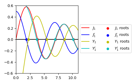
Построить график \(J_1\), \(J_1'\), \(Y_1\), \(Y_1'\) и их корни.

>>> import numpy as np
>>> import matplotlib.pyplot as plt
>>> from scipy.special import jnyn_zeros, jvp, jn, yvp, yn
>>> jn_roots, jnp_roots, yn_roots, ynp_roots = jnyn_zeros(1, 3)
>>> fig, ax = plt.subplots()
>>> xmax= 11
>>> x = np.linspace(0, xmax)
>>> x[0] += 1e-15
>>> ax.plot(x, jn(1, x), label=r"$J_1$", c='r')
>>> ax.plot(x, jvp(1, x, 1), label=r"$J_1'$", c='b')
>>> ax.plot(x, yn(1, x), label=r"$Y_1$", c='y')
>>> ax.plot(x, yvp(1, x, 1), label=r"$Y_1'$", c='c')
>>> zeros = np.zeros((3, ))
>>> ax.scatter(jn_roots, zeros, s=30, c='r', zorder=5,
...            label=r"$J_1$ roots")
>>> ax.scatter(jnp_roots, zeros, s=30, c='b', zorder=5,
...            label=r"$J_1'$ roots")
>>> ax.scatter(yn_roots, zeros, s=30, c='y', zorder=5,
...            label=r"$Y_1$ roots")
>>> ax.scatter(ynp_roots, zeros, s=30, c='c', zorder=5,
...            label=r"$Y_1'$ roots")
>>> ax.hlines(0, 0, xmax, color='k')
>>> ax.set_ylim(-0.6, 0.6)
>>> ax.set_xlim(0, xmax)
>>> ax.legend(ncol=2, bbox_to_anchor=(1., 0.75))
>>> plt.tight_layout()
>>> plt.show()

НазадОткрыть во вкладке