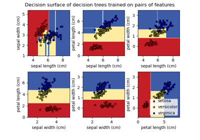
Построить поверхности решений ансамблей деревьев на наборе данных ирисов

Построить поверхности решений лесов рандомизированных деревьев, обученных на парах признаков набора данных ирисов.

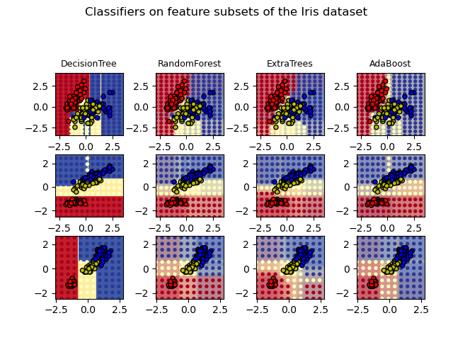
Этот график сравнивает поверхности решений, изученные классификатором дерева решений (первый столбец), классификатором случайного леса (второй столбец), классификатором экстра-деревьев (третий столбец) и классификатором AdaBoost (четвертый столбец).

В первой строке классификаторы построены с использованием только признаков ширины чашелистика и длины чашелистика, во второй строке — только длины лепестка и длины чашелистика, а в третьей строке — только ширины лепестка и длины лепестка.

В порядке убывания качества, при обучении (вне этого примера) на всех 4 признаках с использованием 30 оценщиков и оценке с помощью 10-кратной перекрестной проверки, мы видим:

ExtraTreesClassifier()  # 0.95 score
RandomForestClassifier()  # 0.94 score
AdaBoost(DecisionTree(max_depth=3))  # 0.94 score
DecisionTree(max_depth=None)  # 0.94 score

Увеличение max_depth для AdaBoost снижает стандартное отклонение оценок (но средняя оценка не улучшается).

Смотрите вывод консоли для дополнительных деталей о каждой модели.

В этом примере вы можете попробовать:

1. изменять max_depth для DecisionTreeClassifier и AdaBoostClassifier, возможно, попробуйте max_depth=3 для DecisionTreeClassifier или max_depth=None для AdaBoostClassifier

2. варьировать n_estimators

Стоит отметить, что RandomForests и ExtraTrees можно обучать параллельно на многих ядрах, так как каждое дерево строится независимо от других. Образцы AdaBoost строятся последовательно и поэтому не используют несколько ядер.

DecisionTree with features [0, 1] has a score of 0.9266666666666666
RandomForest with 30 estimators with features [0, 1] has a score of 0.9266666666666666
ExtraTrees with 30 estimators with features [0, 1] has a score of 0.9266666666666666
AdaBoost with 30 estimators with features [0, 1] has a score of 0.82
DecisionTree with features [0, 2] has a score of 0.9933333333333333
RandomForest with 30 estimators with features [0, 2] has a score of 0.9933333333333333
ExtraTrees with 30 estimators with features [0, 2] has a score of 0.9933333333333333
AdaBoost with 30 estimators with features [0, 2] has a score of 0.9933333333333333
DecisionTree with features [2, 3] has a score of 0.9933333333333333
RandomForest with 30 estimators with features [2, 3] has a score of 0.9933333333333333
ExtraTrees with 30 estimators with features [2, 3] has a score of 0.9933333333333333
AdaBoost with 30 estimators with features [2, 3] has a score of 0.9866666666666667

# Authors: The scikit-learn developers
# SPDX-License-Identifier: BSD-3-Clause

import matplotlib.pyplot as plt
import numpy as np
from matplotlib.colors import ListedColormap

from sklearn.datasets import load_iris
from sklearn.ensemble import (
    AdaBoostClassifier,
    ExtraTreesClassifier,
    RandomForestClassifier,
)
from sklearn.tree import DecisionTreeClassifier

# Parameters
n_classes = 3
n_estimators = 30
cmap = plt.cm.RdYlBu
plot_step = 0.02  # fine step width for decision surface contours
plot_step_coarser = 0.5  # step widths for coarse classifier guesses
RANDOM_SEED = 13  # fix the seed on each iteration

# Load data
iris = load_iris()

plot_idx = 1

models = [
    DecisionTreeClassifier(max_depth=None),
    RandomForestClassifier(n_estimators=n_estimators),
    ExtraTreesClassifier(n_estimators=n_estimators),
    AdaBoostClassifier(DecisionTreeClassifier(max_depth=3), n_estimators=n_estimators),
]

for pair in ([0, 1], [0, 2], [2, 3]):
    for model in models:
        # We only take the two corresponding features
        X = iris.data[:, pair]
        y = iris.target

        # Shuffle
        idx = np.arange(X.shape[0])
        np.random.seed(RANDOM_SEED)
        np.random.shuffle(idx)
        X = X[idx]
        y = y[idx]

        # Standardize
        mean = X.mean(axis=0)
        std = X.std(axis=0)
        X = (X - mean) / std

        # Train
        model.fit(X, y)

        scores = model.score(X, y)
        # Create a title for each column and the console by using str() and
        # slicing away useless parts of the string
        model_title = str(type(model)).split(".")[-1][:-2][: -len("Classifier")]

        model_details = model_title
        if hasattr(model, "estimators_"):
            model_details += " with {} estimators".format(len(model.estimators_))
        print(model_details + " with features", pair, "has a score of", scores)

        plt.subplot(3, 4, plot_idx)
        if plot_idx <= len(models):
            # Add a title at the top of each column
            plt.title(model_title, fontsize=9)

        # Now plot the decision boundary using a fine mesh as input to a
        # filled contour plot
        x_min, x_max = X[:, 0].min() - 1, X[:, 0].max() + 1
        y_min, y_max = X[:, 1].min() - 1, X[:, 1].max() + 1
        xx, yy = np.meshgrid(
            np.arange(x_min, x_max, plot_step), np.arange(y_min, y_max, plot_step)
        )

        # Plot either a single DecisionTreeClassifier or alpha blend the
        # decision surfaces of the ensemble of classifiers
        if isinstance(model, DecisionTreeClassifier):
            Z = model.predict(np.c_[xx.ravel(), yy.ravel()])
            Z = Z.reshape(xx.shape)
            cs = plt.contourf(xx, yy, Z, cmap=cmap)
        else:
            # Choose alpha blend level with respect to the number
            # of estimators
            # that are in use (noting that AdaBoost can use fewer estimators
            # than its maximum if it achieves a good enough fit early on)
            estimator_alpha = 1.0 / len(model.estimators_)
            for tree in model.estimators_:
                Z = tree.predict(np.c_[xx.ravel(), yy.ravel()])
                Z = Z.reshape(xx.shape)
                cs = plt.contourf(xx, yy, Z, alpha=estimator_alpha, cmap=cmap)

        # Build a coarser grid to plot a set of ensemble classifications
        # to show how these are different to what we see in the decision
        # surfaces. These points are regularly space and do not have a
        # black outline
        xx_coarser, yy_coarser = np.meshgrid(
            np.arange(x_min, x_max, plot_step_coarser),
            np.arange(y_min, y_max, plot_step_coarser),
        )
        Z_points_coarser = model.predict(
            np.c_[xx_coarser.ravel(), yy_coarser.ravel()]
        ).reshape(xx_coarser.shape)
        cs_points = plt.scatter(
            xx_coarser,
            yy_coarser,
            s=15,
            c=Z_points_coarser,
            cmap=cmap,
            edgecolors="none",
        )

        # Plot the training points, these are clustered together and have a
        # black outline
        plt.scatter(
            X[:, 0],
            X[:, 1],
            c=y,
            cmap=ListedColormap(["r", "y", "b"]),
            edgecolor="k",
            s=20,
        )
        plot_idx += 1  # move on to the next plot in sequence

plt.suptitle("Classifiers on feature subsets of the Iris dataset", fontsize=12)
plt.axis("tight")
plt.tight_layout(h_pad=0.2, w_pad=0.2, pad=2.5)
plt.show()

Связанные примеры

Гауссовский процесс классификации (GPC) на наборе данных iris

Гауссовский процесс классификации (GPC) на наборе данных iris

Изменение регуляризации в многослойном перцептроне

Изменение регуляризации в многослойном перцептроне

Построить поверхность решений деревьев решений, обученных на наборе данных ирисов

Построить поверхность решений деревьев решений, обученных на наборе данных ирисов

SGD: Взвешенные выборки

SGD: Взвешенные выборки