Примечание
Перейти в конец чтобы скачать полный пример кода или запустить этот пример в браузере через JupyterLite или Binder.
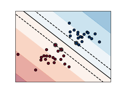
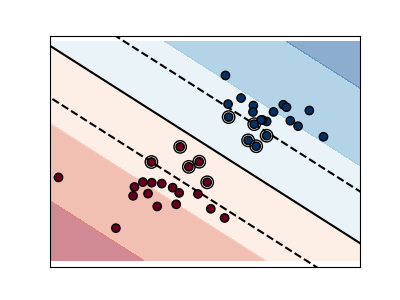
Пример границ SVM#
Графики ниже иллюстрируют влияние параметра C имеет на разделительной линии. Большое значение C по сути говорит нашей модели, что мы не очень доверяем распределению наших данных и будем рассматривать только точки, близкие к линии разделения.
Малое значение C включает больше/все наблюдения, позволяя вычислять поля с использованием всех данных в области.
# Authors: The scikit-learn developers
# SPDX-License-Identifier: BSD-3-Clause

import matplotlib.pyplot as plt
import numpy as np

from sklearn import svm

# we create 40 separable points
np.random.seed(0)
X = np.r_[np.random.randn(20, 2) - [2, 2], np.random.randn(20, 2) + [2, 2]]
Y = [0] * 20 + [1] * 20

# figure number
fignum = 1

# fit the model
for name, penalty in (("unreg", 1), ("reg", 0.05)):
    clf = svm.SVC(kernel="linear", C=penalty)
    clf.fit(X, Y)

    # get the separating hyperplane
    w = clf.coef_[0]
    a = -w[0] / w[1]
    xx = np.linspace(-5, 5)
    yy = a * xx - (clf.intercept_[0]) / w[1]

    # plot the parallels to the separating hyperplane that pass through the
    # support vectors (margin away from hyperplane in direction
    # perpendicular to hyperplane). This is sqrt(1+a^2) away vertically in
    # 2-d.
    margin = 1 / np.sqrt(np.sum(clf.coef_**2))
    yy_down = yy - np.sqrt(1 + a**2) * margin
    yy_up = yy + np.sqrt(1 + a**2) * margin

    # plot the line, the points, and the nearest vectors to the plane
    plt.figure(fignum, figsize=(4, 3))
    plt.clf()
    plt.plot(xx, yy, "k-")
    plt.plot(xx, yy_down, "k--")
    plt.plot(xx, yy_up, "k--")

    plt.scatter(
        clf.support_vectors_[:, 0],
        clf.support_vectors_[:, 1],
        s=80,
        facecolors="none",
        zorder=10,
        edgecolors="k",
    )
    plt.scatter(
        X[:, 0], X[:, 1], c=Y, zorder=10, cmap=plt.get_cmap("RdBu"), edgecolors="k"
    )

    plt.axis("tight")
    x_min = -4.8
    x_max = 4.2
    y_min = -6
    y_max = 6

    YY, XX = np.meshgrid(yy, xx)
    xy = np.vstack([XX.ravel(), YY.ravel()]).T
    Z = clf.decision_function(xy).reshape(XX.shape)

    # Put the result into a contour plot
    plt.contourf(XX, YY, Z, cmap=plt.get_cmap("RdBu"), alpha=0.5, linestyles=["-"])

    plt.xlim(x_min, x_max)
    plt.ylim(y_min, y_max)

    plt.xticks(())
    plt.yticks(())
    fignum = fignum + 1

plt.show()
Общее время выполнения скрипта: (0 минут 0.052 секунды)
Связанные примеры
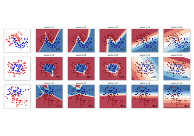
Изменение регуляризации в многослойном перцептроне
Изменение регуляризации в многослойном перцептроне
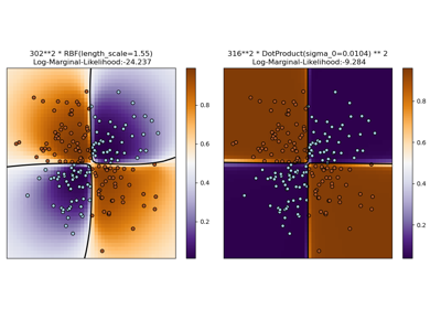
Иллюстрация классификации гауссовским процессом (GPC) на наборе данных XOR
Иллюстрация классификации гауссовским процессом (GPC) на наборе данных XOR
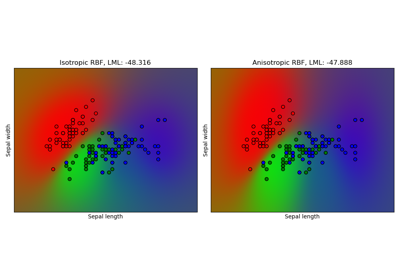
Гауссовский процесс классификации (GPC) на наборе данных iris
Гауссовский процесс классификации (GPC) на наборе данных iris