Примечание

Перейти в конец чтобы скачать полный пример кода или запустить этот пример в браузере через JupyterLite или Binder.

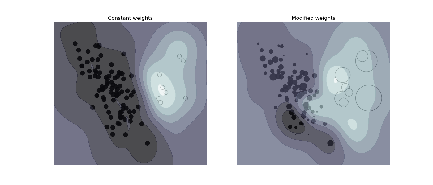
SVM: Взвешенные образцы#

Построить функцию решения для взвешенного набора данных, где размер точек пропорционален их весу.

Взвешивание образцов перемасштабирует параметр C, что означает, что классификатор уделяет больше внимания правильности этих точек. Эффект часто может быть тонким. Чтобы подчеркнуть эффект здесь, мы особенно увеличиваем вес положительного класса, делая деформацию границы решения более заметной.

# Authors: The scikit-learn developers
# SPDX-License-Identifier: BSD-3-Clause

import matplotlib.pyplot as plt
import numpy as np

from sklearn.datasets import make_classification
from sklearn.inspection import DecisionBoundaryDisplay
from sklearn.svm import SVC

X, y = make_classification(
    n_samples=1_000,
    n_features=2,
    n_informative=2,
    n_redundant=0,
    n_clusters_per_class=1,
    class_sep=1.1,
    weights=[0.9, 0.1],
    random_state=0,
)
# down-sample for plotting
rng = np.random.RandomState(0)
plot_indices = rng.choice(np.arange(X.shape[0]), size=100, replace=True)
X_plot, y_plot = X[plot_indices], y[plot_indices]


def plot_decision_function(classifier, sample_weight, axis, title):
    """Plot the synthetic data and the classifier decision function. Points with
    larger sample_weight are mapped to larger circles in the scatter plot."""
    axis.scatter(
        X_plot[:, 0],
        X_plot[:, 1],
        c=y_plot,
        s=100 * sample_weight[plot_indices],
        alpha=0.9,
        cmap=plt.cm.bone,
        edgecolors="black",
    )
    DecisionBoundaryDisplay.from_estimator(
        classifier,
        X_plot,
        response_method="decision_function",
        alpha=0.75,
        ax=axis,
        cmap=plt.cm.bone,
    )
    axis.axis("off")
    axis.set_title(title)


# we define constant weights as expected by the plotting function
sample_weight_constant = np.ones(len(X))
# assign random weights to all points
sample_weight_modified = abs(rng.randn(len(X)))
# assign bigger weights to the positive class
positive_class_indices = np.asarray(y == 1).nonzero()[0]
sample_weight_modified[positive_class_indices] *= 15

# This model does not include sample weights.
clf_no_weights = SVC(gamma=1)
clf_no_weights.fit(X, y)

# This other model includes sample weights.
clf_weights = SVC(gamma=1)
clf_weights.fit(X, y, sample_weight=sample_weight_modified)

fig, axes = plt.subplots(1, 2, figsize=(14, 6))
plot_decision_function(
    clf_no_weights, sample_weight_constant, axes[0], "Constant weights"
)
plot_decision_function(clf_weights, sample_weight_modified, axes[1], "Modified weights")

plt.show()