Пример распознавания лиц с использованием собственных лиц и SVM

Набор данных, используемый в этом примере, представляет собой предобработанный отрывок из «Labeled Faces in the Wild», также известного как LFW: https://www.kaggle.com/datasets/jessicali9530/lfw-dataset

# Authors: The scikit-learn developers
# SPDX-License-Identifier: BSD-3-Clause

from time import time

import matplotlib.pyplot as plt
from scipy.stats import loguniform

from sklearn.datasets import fetch_lfw_people
from sklearn.decomposition import PCA
from sklearn.metrics import ConfusionMatrixDisplay, classification_report
from sklearn.model_selection import RandomizedSearchCV, train_test_split
from sklearn.preprocessing import StandardScaler
from sklearn.svm import SVC

Загрузите данные, если они еще не на диске, и загрузите их как массивы numpy

lfw_people = fetch_lfw_people(min_faces_per_person=70, resize=0.4)

# introspect the images arrays to find the shapes (for plotting)
n_samples, h, w = lfw_people.images.shape

# for machine learning we use the 2 data directly (as relative pixel
# positions info is ignored by this model)
X = lfw_people.data
n_features = X.shape[1]

# the label to predict is the id of the person
y = lfw_people.target
target_names = lfw_people.target_names
n_classes = target_names.shape[0]

print("Total dataset size:")
print("n_samples: %d" % n_samples)
print("n_features: %d" % n_features)
print("n_classes: %d" % n_classes)

Total dataset size:
n_samples: 1288
n_features: 1850
n_classes: 7

Разделить на обучающий набор и тестовый набор, оставив 25% данных для тестирования.

X_train, X_test, y_train, y_test = train_test_split(
    X, y, test_size=0.25, random_state=42
)

scaler = StandardScaler()
X_train = scaler.fit_transform(X_train)
X_test = scaler.transform(X_test)

Вычисление PCA (собственных лиц) на наборе данных лиц (рассматриваемом как неразмеченный набор данных): извлечение признаков без учителя / уменьшение размерности

n_components = 150

print(
    "Extracting the top %d eigenfaces from %d faces" % (n_components, X_train.shape[0])
)
t0 = time()
pca = PCA(n_components=n_components, svd_solver="randomized", whiten=True).fit(X_train)
print("done in %0.3fs" % (time() - t0))

eigenfaces = pca.components_.reshape((n_components, h, w))

print("Projecting the input data on the eigenfaces orthonormal basis")
t0 = time()
X_train_pca = pca.transform(X_train)
X_test_pca = pca.transform(X_test)
print("done in %0.3fs" % (time() - t0))

Extracting the top 150 eigenfaces from 966 faces
done in 0.100s
Projecting the input data on the eigenfaces orthonormal basis
done in 0.006s

Обучить модель классификации SVM

print("Fitting the classifier to the training set")
t0 = time()
param_grid = {
    "C": loguniform(1e3, 1e5),
    "gamma": loguniform(1e-4, 1e-1),
}
clf = RandomizedSearchCV(
    SVC(kernel="rbf", class_weight="balanced"), param_grid, n_iter=10
)
clf = clf.fit(X_train_pca, y_train)
print("done in %0.3fs" % (time() - t0))
print("Best estimator found by grid search:")
print(clf.best_estimator_)

Fitting the classifier to the training set
done in 6.191s
Best estimator found by grid search:
SVC(C=np.float64(76823.03433306457), class_weight='balanced',
    gamma=np.float64(0.0034189458230957995))

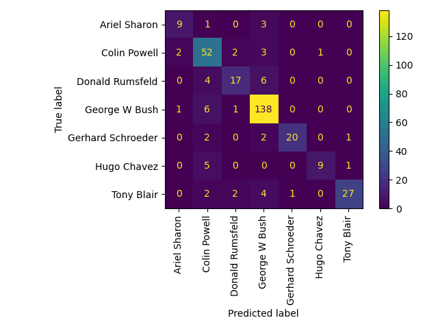
Количественная оценка качества модели на тестовом наборе

print("Predicting people's names on the test set")
t0 = time()
y_pred = clf.predict(X_test_pca)
print("done in %0.3fs" % (time() - t0))

print(classification_report(y_test, y_pred, target_names=target_names))
ConfusionMatrixDisplay.from_estimator(
    clf, X_test_pca, y_test, display_labels=target_names, xticks_rotation="vertical"
)
plt.tight_layout()
plt.show()

Predicting people's names on the test set
done in 0.046s
                   precision    recall  f1-score   support

     Ariel Sharon       0.75      0.69      0.72        13
     Colin Powell       0.72      0.87      0.79        60
  Donald Rumsfeld       0.77      0.63      0.69        27
    George W Bush       0.88      0.95      0.91       146
Gerhard Schroeder       0.95      0.80      0.87        25
      Hugo Chavez       0.90      0.60      0.72        15
       Tony Blair       0.93      0.75      0.83        36

         accuracy                           0.84       322
        macro avg       0.84      0.75      0.79       322
     weighted avg       0.85      0.84      0.84       322

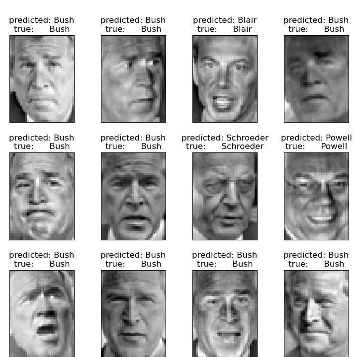
Качественная оценка предсказаний с использованием matplotlib

def plot_gallery(images, titles, h, w, n_row=3, n_col=4):
    """Helper function to plot a gallery of portraits"""
    plt.figure(figsize=(1.8 * n_col, 2.4 * n_row))
    plt.subplots_adjust(bottom=0, left=0.01, right=0.99, top=0.90, hspace=0.35)
    for i in range(n_row * n_col):
        plt.subplot(n_row, n_col, i + 1)
        plt.imshow(images[i].reshape((h, w)), cmap=plt.cm.gray)
        plt.title(titles[i], size=12)
        plt.xticks(())
        plt.yticks(())

построить график результата предсказания на части тестового набора

def title(y_pred, y_test, target_names, i):
    pred_name = target_names[y_pred[i]].rsplit(" ", 1)[-1]
    true_name = target_names[y_test[i]].rsplit(" ", 1)[-1]
    return "predicted: %s\ntrue:      %s" % (pred_name, true_name)


prediction_titles = [
    title(y_pred, y_test, target_names, i) for i in range(y_pred.shape[0])
]

plot_gallery(X_test, prediction_titles, h, w)

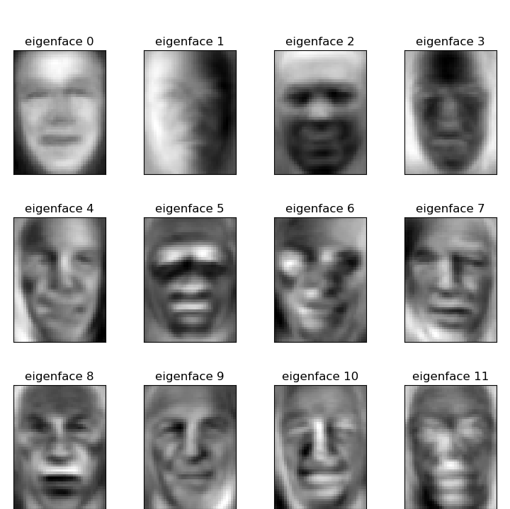
построить галерею наиболее значимых собственных лиц

eigenface_titles = ["eigenface %d" % i for i in range(eigenfaces.shape[0])]
plot_gallery(eigenfaces, eigenface_titles, h, w)

plt.show()

Проблема распознавания лиц была бы гораздо эффективнее решена обучением сверточных нейронных сетей, но это семейство моделей выходит за рамки библиотеки scikit-learn. Заинтересованным читателям следует попробовать использовать pytorch или tensorflow для реализации таких моделей.

Связанные примеры

Извлечение тем с использованием неотрицательной матричной факторизации и латентного размещения Дирихле

Извлечение тем с использованием неотрицательной матричной факторизации и латентного размещения Дирихле

Классификация текстовых документов с использованием разреженных признаков

Классификация текстовых документов с использованием разреженных признаков

Онлайн-обучение словаря частей лиц

Онлайн-обучение словаря частей лиц

Агломерация признаков

Агломерация признаков