Примечание
Перейти в конец чтобы скачать полный пример кода или запустить этот пример в браузере через JupyterLite или Binder.
Выбор количества кластеров с помощью анализа силуэта для кластеризации KMeans#
Анализ силуэтов может использоваться для изучения расстояния разделения между полученными кластерами. График силуэтов отображает меру того, насколько каждая точка в одном кластере близка к точкам в соседних кластерах, и таким образом предоставляет способ визуальной оценки параметров, таких как количество кластеров. Эта мера имеет диапазон [-1, 1].
Коэффициенты силуэта (так называются эти значения) близкие к +1 указывают на то, что выборка далека от соседних кластеров. Значение 0 указывает, что выборка находится на границе принятия решения между двумя соседними кластерами или очень близко к ней, а отрицательные значения указывают, что эти выборки могли быть неправильно отнесены к кластеру.
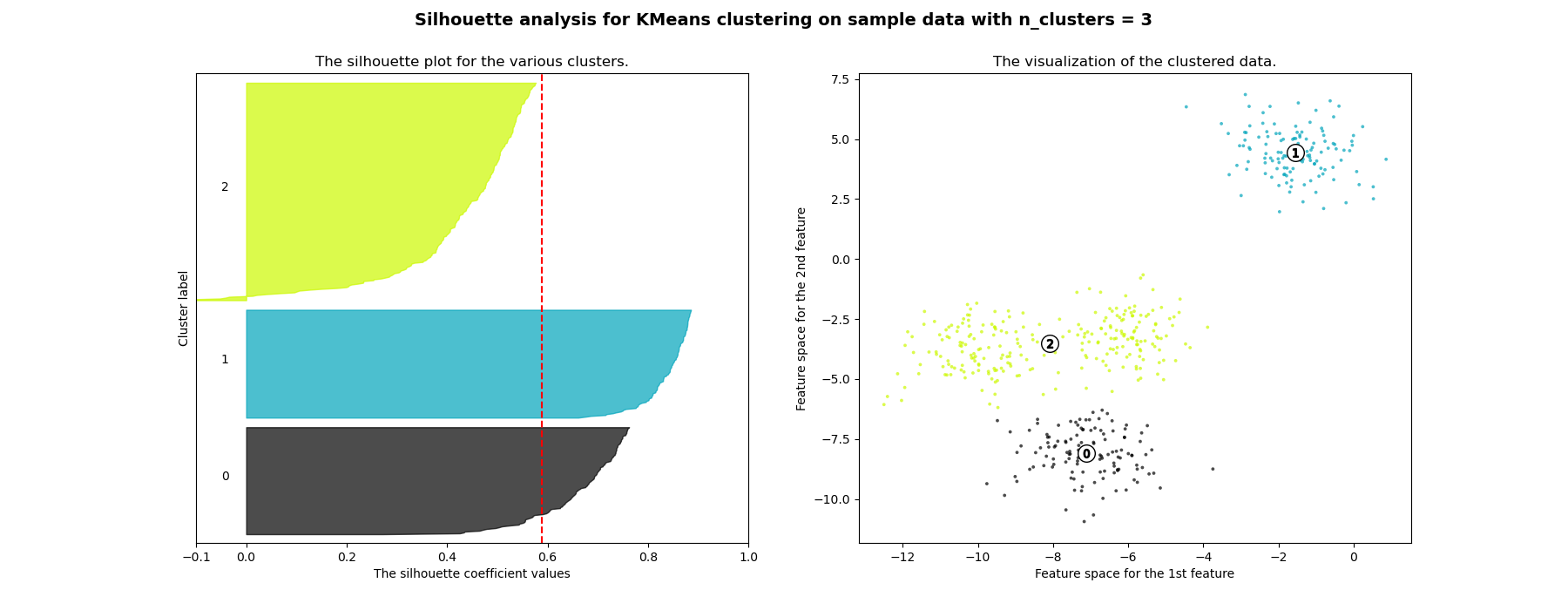
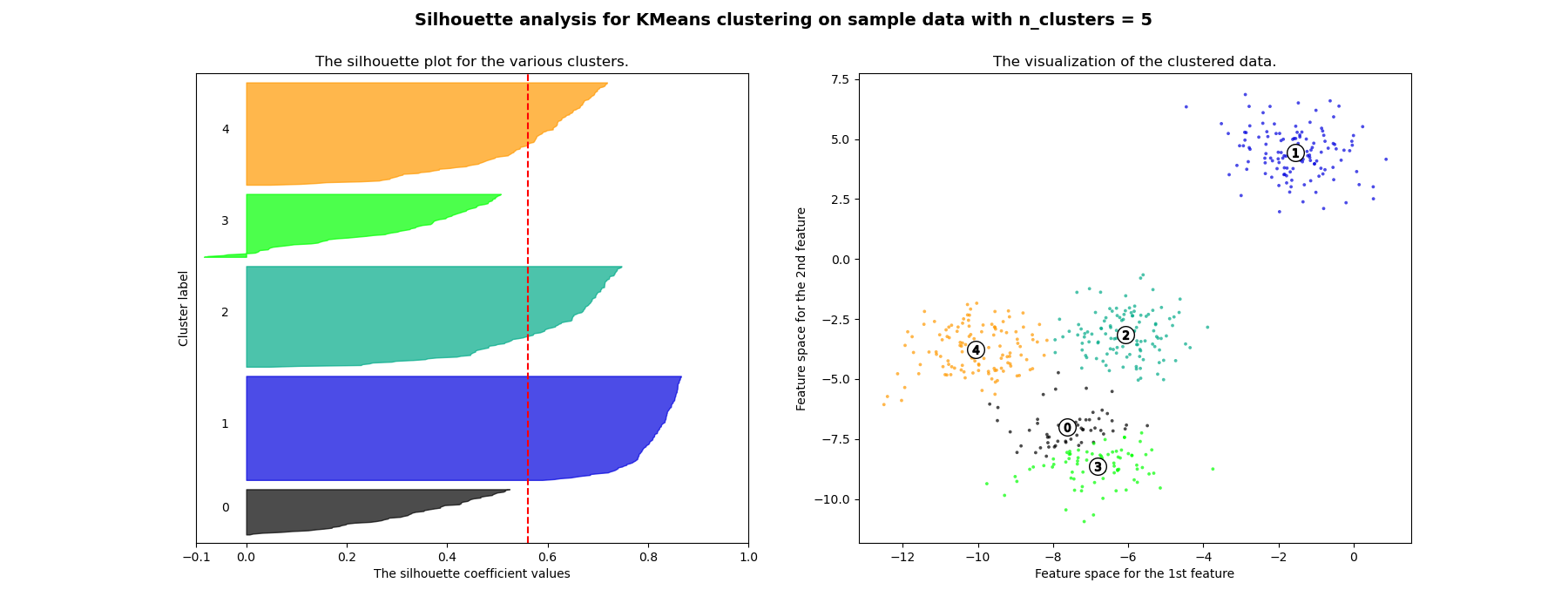
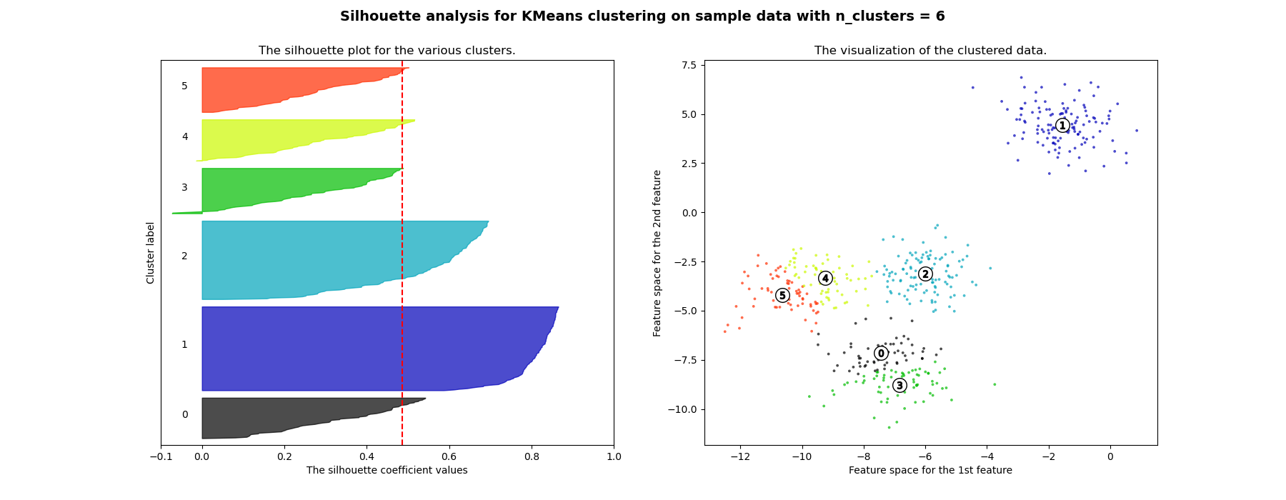
В этом примере анализ силуэта используется для выбора оптимального значения для
n_clusters. График силуэта показывает, что n_clusters значения 3, 5
и 6 являются плохим выбором для данных из-за наличия кластеров с
ниже среднего оценками силуэта, а также из-за широких колебаний в размере
графиков силуэта. Анализ силуэта более неоднозначен при выборе
между 2 и 4.
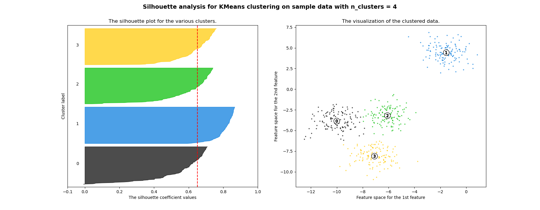
Также по толщине графика силуэта можно визуализировать размер кластера. График силуэта для кластера 0, когда n_clusters равно 2, больше по размеру из-за объединения 3 подкластеров в один большой кластер. Однако, когда n_clusters равна 4, все графики более или менее одинаковой толщины и, следовательно, имеют схожие размеры, что также можно проверить по помеченной диаграмме рассеяния справа.
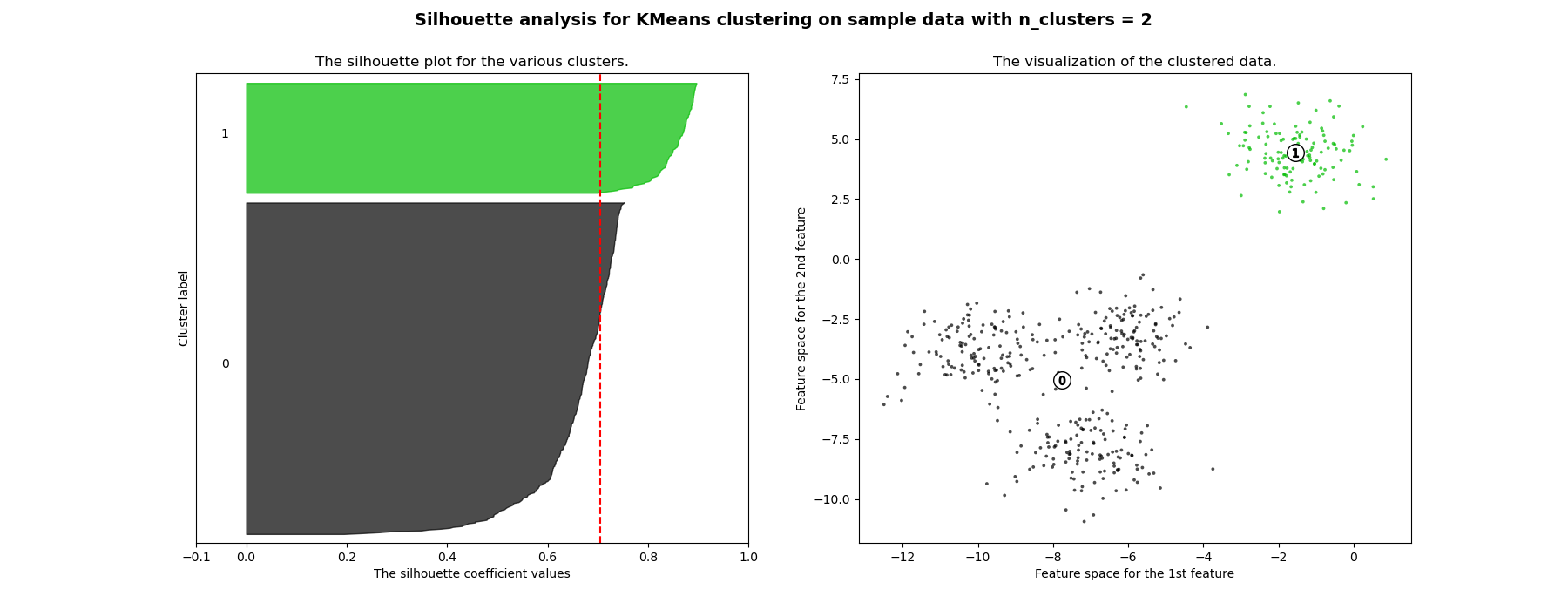
For n_clusters = 2 The average silhouette_score is : 0.7049787496083262
For n_clusters = 3 The average silhouette_score is : 0.5882004012129721
For n_clusters = 4 The average silhouette_score is : 0.6505186632729437
For n_clusters = 5 The average silhouette_score is : 0.561464362648773
For n_clusters = 6 The average silhouette_score is : 0.4857596147013469
# Authors: The scikit-learn developers
# SPDX-License-Identifier: BSD-3-Clause
import matplotlib.cm as cm
import matplotlib.pyplot as plt
import numpy as np
from sklearn.cluster import KMeans
from sklearn.datasets import make_blobs
from sklearn.metrics import silhouette_samples, silhouette_score
# Generating the sample data from make_blobs
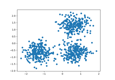
# This particular setting has one distinct cluster and 3 clusters placed close
# together.
X, y = make_blobs(
n_samples=500,
n_features=2,
centers=4,
cluster_std=1,
center_box=(-10.0, 10.0),
shuffle=True,
random_state=1,
) # For reproducibility
range_n_clusters = [2, 3, 4, 5, 6]
for n_clusters in range_n_clusters:
# Create a subplot with 1 row and 2 columns
fig, (ax1, ax2) = plt.subplots(1, 2)
fig.set_size_inches(18, 7)
# The 1st subplot is the silhouette plot
# The silhouette coefficient can range from -1, 1 but in this example all
# lie within [-0.1, 1]
ax1.set_xlim([-0.1, 1])
# The (n_clusters+1)*10 is for inserting blank space between silhouette
# plots of individual clusters, to demarcate them clearly.
ax1.set_ylim([0, len(X) + (n_clusters + 1) * 10])
# Initialize the clusterer with n_clusters value and a random generator
# seed of 10 for reproducibility.
clusterer = KMeans(n_clusters=n_clusters, random_state=10)
cluster_labels = clusterer.fit_predict(X)
# The silhouette_score gives the average value for all the samples.
# This gives a perspective into the density and separation of the formed
# clusters
silhouette_avg = silhouette_score(X, cluster_labels)
print(
"For n_clusters =",
n_clusters,
"The average silhouette_score is :",
silhouette_avg,
)
# Compute the silhouette scores for each sample
sample_silhouette_values = silhouette_samples(X, cluster_labels)
y_lower = 10
for i in range(n_clusters):
# Aggregate the silhouette scores for samples belonging to
# cluster i, and sort them
ith_cluster_silhouette_values = sample_silhouette_values[cluster_labels == i]
ith_cluster_silhouette_values.sort()
size_cluster_i = ith_cluster_silhouette_values.shape[0]
y_upper = y_lower + size_cluster_i
color = cm.nipy_spectral(float(i) / n_clusters)
ax1.fill_betweenx(
np.arange(y_lower, y_upper),
0,
ith_cluster_silhouette_values,
facecolor=color,
edgecolor=color,
alpha=0.7,
)
# Label the silhouette plots with their cluster numbers at the middle
ax1.text(-0.05, y_lower + 0.5 * size_cluster_i, str(i))
# Compute the new y_lower for next plot
y_lower = y_upper + 10 # 10 for the 0 samples
ax1.set_title("The silhouette plot for the various clusters.")
ax1.set_xlabel("The silhouette coefficient values")
ax1.set_ylabel("Cluster label")
# The vertical line for average silhouette score of all the values
ax1.axvline(x=silhouette_avg, color="red", linestyle="--")
ax1.set_yticks([]) # Clear the yaxis labels / ticks
ax1.set_xticks([-0.1, 0, 0.2, 0.4, 0.6, 0.8, 1])
# 2nd Plot showing the actual clusters formed
colors = cm.nipy_spectral(cluster_labels.astype(float) / n_clusters)
ax2.scatter(
X[:, 0], X[:, 1], marker=".", s=30, lw=0, alpha=0.7, c=colors, edgecolor="k"
)
# Labeling the clusters
centers = clusterer.cluster_centers_
# Draw white circles at cluster centers
ax2.scatter(
centers[:, 0],
centers[:, 1],
marker="o",
c="white",
alpha=1,
s=200,
edgecolor="k",
)
for i, c in enumerate(centers):
ax2.scatter(c[0], c[1], marker="$%d$" % i, alpha=1, s=50, edgecolor="k")
ax2.set_title("The visualization of the clustered data.")
ax2.set_xlabel("Feature space for the 1st feature")
ax2.set_ylabel("Feature space for the 2nd feature")
plt.suptitle(
"Silhouette analysis for KMeans clustering on sample data with n_clusters = %d"
% n_clusters,
fontsize=14,
fontweight="bold",
)
plt.show()
Общее время выполнения скрипта: (0 минут 0.905 секунд)
Связанные примеры
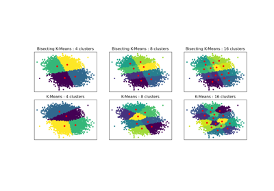
Сравнение производительности биссекционного K-средних и обычного K-средних
Кластеризация текстовых документов с использованием k-means