Примечание
Перейти в конец чтобы скачать полный пример кода или запустить этот пример в браузере через JupyterLite или Binder.
Калибровка вероятностей классификаторов#
При выполнении классификации часто хочется предсказать не только метку класса, но и связанную с ней вероятность. Эта вероятность даёт некоторую уверенность в предсказании. Однако не все классификаторы предоставляют хорошо калиброванные вероятности: некоторые слишком уверены, а другие недостаточно уверены. Поэтому часто желательна отдельная калибровка предсказанных вероятностей как постобработка. Этот пример иллюстрирует два различных метода такой калибровки и оценивает качество возвращаемых вероятностей с помощью оценки Брайера (см. https://en.wikipedia.org/wiki/Brier_score).
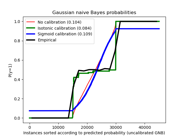
Сравниваются оценённые вероятности с использованием наивного байесовского классификатора Гаусса без калибровки, с сигмоидной калибровкой и с непараметрической изотонной калибровкой. Можно заметить, что только непараметрическая модель способна обеспечить калибровку вероятностей, которая возвращает вероятности, близкие к ожидаемым 0.5 для большинства образцов, принадлежащих среднему кластеру с неоднородными метками. Это приводит к значительному улучшению оценки Брайера.
# Authors: The scikit-learn developers
# SPDX-License-Identifier: BSD-3-Clause
Сгенерировать синтетический набор данных#
import numpy as np

from sklearn.datasets import make_blobs
from sklearn.model_selection import train_test_split

n_samples = 50000

# Generate 3 blobs with 2 classes where the second blob contains
# half positive samples and half negative samples. Probability in this
# blob is therefore 0.5.
centers = [(-5, -5), (0, 0), (5, 5)]
X, y = make_blobs(n_samples=n_samples, centers=centers, shuffle=False, random_state=42)

y[: n_samples // 2] = 0
y[n_samples // 2 :] = 1
sample_weight = np.random.RandomState(42).rand(y.shape[0])

# split train, test for calibration
X_train, X_test, y_train, y_test, sw_train, sw_test = train_test_split(
    X, y, sample_weight, test_size=0.9, random_state=42
)
Гауссовский наивный байесовский классификатор#
from sklearn.calibration import CalibratedClassifierCV
from sklearn.metrics import brier_score_loss
from sklearn.naive_bayes import GaussianNB

# With no calibration
clf = GaussianNB()
clf.fit(X_train, y_train)  # GaussianNB itself does not support sample-weights
prob_pos_clf = clf.predict_proba(X_test)[:, 1]

# With isotonic calibration
clf_isotonic = CalibratedClassifierCV(clf, cv=2, method="isotonic")
clf_isotonic.fit(X_train, y_train, sample_weight=sw_train)
prob_pos_isotonic = clf_isotonic.predict_proba(X_test)[:, 1]

# With sigmoid calibration
clf_sigmoid = CalibratedClassifierCV(clf, cv=2, method="sigmoid")
clf_sigmoid.fit(X_train, y_train, sample_weight=sw_train)
prob_pos_sigmoid = clf_sigmoid.predict_proba(X_test)[:, 1]

print("Brier score losses: (the smaller the better)")

clf_score = brier_score_loss(y_test, prob_pos_clf, sample_weight=sw_test)
print("No calibration: %1.3f" % clf_score)

clf_isotonic_score = brier_score_loss(y_test, prob_pos_isotonic, sample_weight=sw_test)
print("With isotonic calibration: %1.3f" % clf_isotonic_score)

clf_sigmoid_score = brier_score_loss(y_test, prob_pos_sigmoid, sample_weight=sw_test)
print("With sigmoid calibration: %1.3f" % clf_sigmoid_score)
Brier score losses: (the smaller the better)
No calibration: 0.104
With isotonic calibration: 0.084
With sigmoid calibration: 0.109
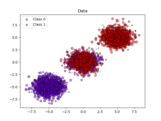
Построить данные и предсказанные вероятности#
import matplotlib.pyplot as plt
from matplotlib import cm

plt.figure()
y_unique = np.unique(y)
colors = cm.rainbow(np.linspace(0.0, 1.0, y_unique.size))
for this_y, color in zip(y_unique, colors):
    this_X = X_train[y_train == this_y]
    this_sw = sw_train[y_train == this_y]
    plt.scatter(
        this_X[:, 0],
        this_X[:, 1],
        s=this_sw * 50,
        c=color[np.newaxis, :],
        alpha=0.5,
        edgecolor="k",
        label="Class %s" % this_y,
    )
plt.legend(loc="best")
plt.title("Data")

plt.figure()

order = np.lexsort((prob_pos_clf,))
plt.plot(prob_pos_clf[order], "r", label="No calibration (%1.3f)" % clf_score)
plt.plot(
    prob_pos_isotonic[order],
    "g",
    linewidth=3,
    label="Isotonic calibration (%1.3f)" % clf_isotonic_score,
)
plt.plot(
    prob_pos_sigmoid[order],
    "b",
    linewidth=3,
    label="Sigmoid calibration (%1.3f)" % clf_sigmoid_score,
)
plt.plot(
    np.linspace(0, y_test.size, 51)[1::2],
    y_test[order].reshape(25, -1).mean(1),
    "k",
    linewidth=3,
    label=r"Empirical",
)
plt.ylim([-0.05, 1.05])
plt.xlabel("Instances sorted according to predicted probability (uncalibrated GNB)")
plt.ylabel("P(y=1)")
plt.legend(loc="upper left")
plt.title("Gaussian naive Bayes probabilities")

plt.show()
Общее время выполнения скрипта: (0 минут 0.406 секунд)
Связанные примеры
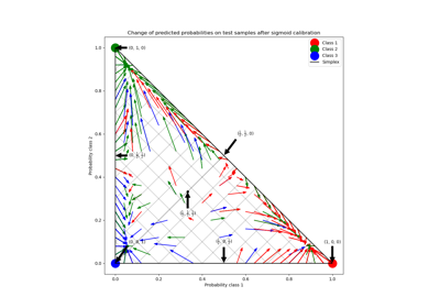
Калибровка вероятностей для классификации на 3 класса