Заполнение пропущенных значений с вариантами IterativeImputer

The IterativeImputer класс очень гибкий - он может использоваться с различными оценщиками для выполнения круговой регрессии, обрабатывая каждую переменную как выход по очереди.

В этом примере мы сравниваем некоторые оценки для целей импутации пропущенных признаков с IterativeImputer:

• BayesianRidge: регуляризованная линейная регрессия

• RandomForestRegressor: регрессия лесов рандомизированных деревьев

• make_pipeline (Nystroem, Ridge): конвейер с расширением полиномиального ядра степени 2 и регуляризованной линейной регрессией

• KNeighborsRegressor: сопоставимо с другими подходами KNN для заполнения пропусков

Особый интерес представляет способность IterativeImputer чтобы имитировать поведение missForest, популярного пакета импутации для R.

Обратите внимание, что KNeighborsRegressor отличается от KNN импутации, которая обучается на образцах с пропущенными значениями, используя метрику расстояния, учитывающую пропущенные значения, а не импутирует их.

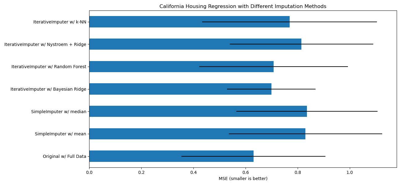
Цель — сравнить различные оценщики, чтобы увидеть, какой из них лучше всего подходит для IterativeImputer при использовании BayesianRidge оценщик на наборе данных California housing с одним случайно удаленным значением из каждой строки.

Для этого конкретного шаблона пропущенных значений мы видим, что BayesianRidge и RandomForestRegressor дают лучшие результаты.

Следует отметить, что некоторые оценщики, такие как HistGradientBoostingRegressor могут изначально работать с пропущенными признаками и часто рекомендуются вместо построения конвейеров со сложными и дорогостоящими стратегиями импутации пропущенных значений.

# Authors: The scikit-learn developers
# SPDX-License-Identifier: BSD-3-Clause

import matplotlib.pyplot as plt
import numpy as np
import pandas as pd

from sklearn.datasets import fetch_california_housing
from sklearn.ensemble import RandomForestRegressor

# To use this experimental feature, we need to explicitly ask for it:
from sklearn.experimental import enable_iterative_imputer  # noqa: F401
from sklearn.impute import IterativeImputer, SimpleImputer
from sklearn.kernel_approximation import Nystroem
from sklearn.linear_model import BayesianRidge, Ridge
from sklearn.model_selection import cross_val_score
from sklearn.neighbors import KNeighborsRegressor
from sklearn.pipeline import make_pipeline
from sklearn.preprocessing import RobustScaler

N_SPLITS = 5

X_full, y_full = fetch_california_housing(return_X_y=True)
# ~2k samples is enough for the purpose of the example.
# Remove the following two lines for a slower run with different error bars.
X_full = X_full[::10]
y_full = y_full[::10]
n_samples, n_features = X_full.shape


def compute_score_for(X, y, imputer=None):
    # We scale data before imputation and training a target estimator,
    # because our target estimator and some of the imputers assume
    # that the features have similar scales.
    if imputer is None:
        estimator = make_pipeline(RobustScaler(), BayesianRidge())
    else:
        estimator = make_pipeline(RobustScaler(), imputer, BayesianRidge())
    return cross_val_score(
        estimator, X, y, scoring="neg_mean_squared_error", cv=N_SPLITS
    )


# Estimate the score on the entire dataset, with no missing values
score_full_data = pd.DataFrame(
    compute_score_for(X_full, y_full),
    columns=["Full Data"],
)

# Add a single missing value to each row
rng = np.random.RandomState(0)
X_missing = X_full.copy()
y_missing = y_full
missing_samples = np.arange(n_samples)
missing_features = rng.choice(n_features, n_samples, replace=True)
X_missing[missing_samples, missing_features] = np.nan

# Estimate the score after imputation (mean and median strategies)
score_simple_imputer = pd.DataFrame()
for strategy in ("mean", "median"):
    score_simple_imputer[strategy] = compute_score_for(
        X_missing, y_missing, SimpleImputer(strategy=strategy)
    )

# Estimate the score after iterative imputation of the missing values
# with different estimators
named_estimators = [
    ("Bayesian Ridge", BayesianRidge()),
    (
        "Random Forest",
        RandomForestRegressor(
            # We tuned the hyperparameters of the RandomForestRegressor to get a good
            # enough predictive performance for a restricted execution time.
            n_estimators=5,
            max_depth=10,
            bootstrap=True,
            max_samples=0.5,
            n_jobs=2,
            random_state=0,
        ),
    ),
    (
        "Nystroem + Ridge",
        make_pipeline(
            Nystroem(kernel="polynomial", degree=2, random_state=0), Ridge(alpha=1e4)
        ),
    ),
    (
        "k-NN",
        KNeighborsRegressor(n_neighbors=10),
    ),
]
score_iterative_imputer = pd.DataFrame()
# Iterative imputer is sensitive to the tolerance and
# dependent on the estimator used internally.
# We tuned the tolerance to keep this example run with limited computational
# resources while not changing the results too much compared to keeping the
# stricter default value for the tolerance parameter.
tolerances = (1e-3, 1e-1, 1e-1, 1e-2)
for (name, impute_estimator), tol in zip(named_estimators, tolerances):
    score_iterative_imputer[name] = compute_score_for(
        X_missing,
        y_missing,
        IterativeImputer(
            random_state=0, estimator=impute_estimator, max_iter=40, tol=tol
        ),
    )

scores = pd.concat(
    [score_full_data, score_simple_imputer, score_iterative_imputer],
    keys=["Original", "SimpleImputer", "IterativeImputer"],
    axis=1,
)

# plot california housing results
fig, ax = plt.subplots(figsize=(13, 6))
means = -scores.mean()
errors = scores.std()
means.plot.barh(xerr=errors, ax=ax)
ax.set_title("California Housing Regression with Different Imputation Methods")
ax.set_xlabel("MSE (smaller is better)")
ax.set_yticks(np.arange(means.shape[0]))
ax.set_yticklabels([" w/ ".join(label) for label in means.index.tolist()])
plt.tight_layout(pad=1)
plt.show()

Связанные примеры

Заполнение пропущенных значений перед построением оценщика

Заполнение пропущенных значений перед построением оценщика

Основные нововведения в выпуске scikit-learn 0.22

Основные нововведения в выпуске scikit-learn 0.22

Объедините предикторы с помощью стекинга

Объедините предикторы с помощью стекинга

Отображение оценщиков и сложных конвейеров

Отображение оценщиков и сложных конвейеров